

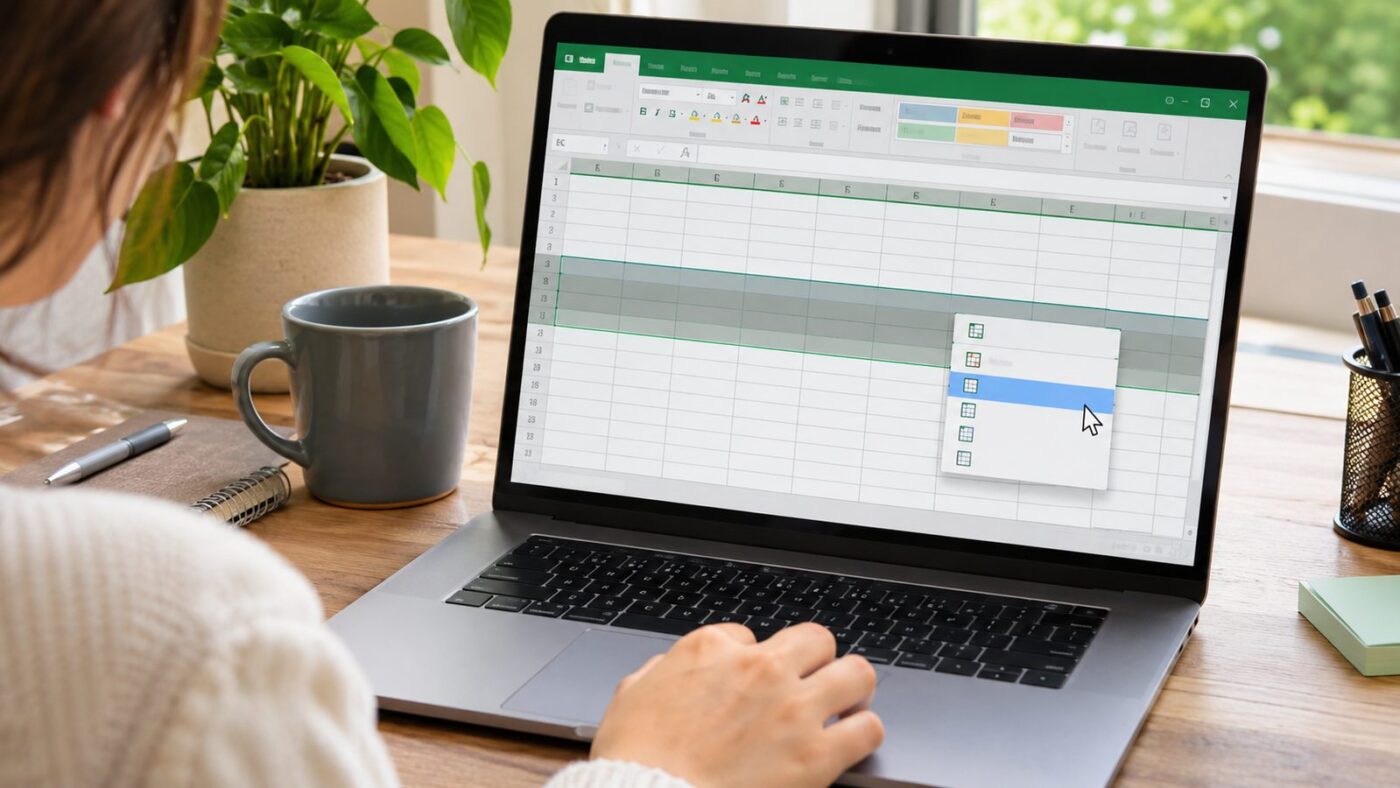
If you need to hide rows in Excel, you can do it without deleting any data. Select the row numbers, right-click them, and choose Hide from the menu. You can also press Ctrl + 9 on Windows for a faster option. Hidden rows remain in your worksheet and can be shown again whenever needed. This makes hiding useful for reports, presentations, and large spreadsheets. It also lets you focus on important information without permanently changing your data. Quick answer: To hide rows, select their row numbers and right-click the selection. Choose Hide, or press Ctrl + 9 on Windows. To restore them, select the rows surrounding the hidden section, right-click, and choose Unhide.
| Task | Fastest method | What happens |
|---|---|---|
| Hide one row | Right-click row number > Hide | Row disappears from view |
| Hide several rows | Select rows > Ctrl + 9 | Selected rows become hidden |
| Hide using Ribbon | Home > Format > Hide & Unhide > Hide Rows | Selected rows become hidden |
| Unhide rows | Select surrounding rows > Unhide | Hidden rows appear again |
| Unhide all rows | Select whole sheet > Unhide Rows | All manually hidden rows appear |
| Hide recurring sections | Data > Group | Creates expandable and collapsible sections |
How to Hide Rows in Excel Step by Step
The simplest method works in current desktop versions of Microsoft Excel. You only need to select the complete row before using the Hide command. Selecting the row number helps prevent accidentally working with individual cells instead.
1. Select the row. Click its numbered heading on the left side of the worksheet. 2. Select additional rows if needed. Drag across adjacent row numbers or use Ctrl-click for separate rows. 3. Right-click the selection. Make sure you right-click a selected row heading. 4. Choose Hide. Excel removes the selected rows from the visible worksheet area.
After hiding a row, its number disappears from the sequence along the worksheet edge. You may see row 5 followed immediately by row 7, for example. That gap indicates that row 6 is hidden rather than deleted. This method is useful when preparing a spreadsheet for another person to read. You can remove distracting detail while keeping the underlying information available. It also avoids making a separate copy of the workbook.
Use the Excel Shortcut to Hide Rows
Keyboard users can hide selected rows without opening a menu. On Windows, Microsoft lists Ctrl + 9 as the shortcut for hiding selected rows. Select the required rows first, then press the shortcut once. This method can save time when you regularly format financial reports or large data tables. It is also useful when your mouse pointer is already inside the selected range. Remember that the shortcut hides complete rows associated with your current selection. If the shortcut appears ineffective, check whether your worksheet selection is correct. Try selecting the row headings directly before pressing the keys again. A protected worksheet can also restrict certain formatting actions.
Hide Rows From the Excel Ribbon
Excel also provides the Hide command through its Ribbon interface. This route can be easier when you do not remember keyboard shortcuts. It also makes the available hide and unhide commands easier to find. First, select the row or rows you want to conceal. Open the Home tab and find the Cells section. Choose Format > Hide & Unhide > Hide Rows to hide your selection. The Ribbon method produces the same basic result as right-clicking the row heading. Your data stays in the workbook while the selected rows disappear visually. You can reverse the change later with the corresponding Unhide Rows command. If Excel skills support your remote career, ReadSnow also covers high-paying remote jobs. Several digital roles rely heavily on spreadsheet and data-management skills. Learning small productivity shortcuts can make routine office work faster.
How to Hide Multiple Rows in Excel
You can hide several adjacent rows in one action. Click the first row number, then drag through the remaining row numbers. After selecting them, right-click and choose Hide. For separate rows, hold Ctrl while selecting individual row numbers on Windows. This lets you select rows that are not next to each other. Apply the Hide command after finishing the selection. Hiding multiple rows can make long reports easier to scan. You might temporarily conceal supporting calculations while displaying totals and key results. The hidden information remains available when you need to review the complete worksheet. This approach is useful for people working across several digital tools each day. ReadSnow’s guide to part-time flexible remote jobs discusses technology-based work across several industries. Spreadsheet organization can help when managing assignments, schedules, or reporting tasks remotely.
How to Unhide Rows in Excel
Unhiding rows is almost as simple as hiding them. Select the visible row immediately above the hidden area and the row immediately below it. Right-click the selected row headings and choose Unhide. Suppose your worksheet jumps from row 10 to row 14. Select row headings 10 through 14 before choosing Unhide. Rows 11, 12, and 13 should then become visible again. You can also use Home > Format > Hide & Unhide > Unhide Rows. This route is helpful when the context menu does not show the expected command. It also works well when you prefer navigating Excel through the Ribbon.
How to Unhide the First Row
Row 1 can be harder to restore because there is no visible row above it. Microsoft recommends selecting cell A1 through the Name Box or Go To command. You can then use the Ribbon’s Unhide Rows option. Type A1 into the Name Box beside the formula bar and press Enter. Next, choose Home > Format > Hide & Unhide > Unhide Rows. The hidden first row should become visible again. Another option is selecting the entire worksheet before applying Unhide Rows. That approach may reveal other hidden rows at the same time. Use the A1 method when you want greater control.
How to Unhide All Rows at Once
Select the whole worksheet when you want every manually hidden row displayed. Click the triangle where the column letters and row numbers meet. You can then open the Ribbon and choose Unhide Rows. This method is useful when reviewing a workbook received from another person. It helps reveal manually hidden information without searching for every missing row number. Remember that filtered rows operate differently from manually hidden rows. For other technology workflows, ReadSnow also explains tools such as the ScanSnap iX1600 document scanner. Document scanning and spreadsheet organization often appear together in paper-to-digital workflows. Both can reduce clutter when records are handled consistently.

Hiding Rows Versus Filtering Rows
Hiding and filtering can make rows disappear, but they solve different problems. Manual hiding works best when you already know which specific rows should disappear. Filtering hides records according to criteria in your data. A filter is usually better when rows must disappear based on values. For example, you could show only orders from California or transactions above $1,000. Clearing the filter restores records that did not match those conditions. Manual hiding is easier for a small, fixed selection. Filtering is more useful when the underlying dataset changes frequently. Choosing the correct method makes your worksheet easier to maintain.
Hiding Rows Versus Grouping Rows
Excel’s Group feature provides another way to temporarily collapse worksheet sections. Grouping adds outline controls that let users expand or collapse a selected range. This can be more convenient than repeatedly hiding and unhiding the same rows. Use grouping when readers may need to switch between detailed and summarized views. It works well for budgets, monthly reports, and structured financial models. Manual hiding works better when you want a cleaner view without visible outline controls. The two features can coexist inside the same workbook. Still, using too many hidden or grouped sections can confuse other users. Keep the worksheet structure predictable when sharing files.
Does Hiding Rows Delete the Data?
No, hiding a row does not delete its contents. The row stays inside the workbook and can be made visible again. Formulas can also continue referencing cells located in hidden rows. This detail matters when you check totals after concealing information. A standard formula may still include values you cannot currently see. Do not assume hidden numbers have stopped affecting calculations. If you need data removed permanently, deleting the row is a different action. Make a backup before deleting important workbook information. Hiding is usually the safer choice when you may need the data later.
Are Hidden Rows Secure?
Hidden rows should not be treated as a privacy or security feature. Another workbook user can usually reveal them with Excel’s Unhide command. Sensitive information should therefore not rely on hiding alone. Remove confidential information before sharing when recipients should never access it. You can also consider workbook permissions and appropriate protection features. The correct approach depends on who receives the file and what access they require. This distinction is particularly important for payroll, customer records, and confidential business reports. A visually hidden row still belongs to the workbook. Treat hiding as a presentation tool rather than an access-control system.
Common Problems When Rows Will Not Unhide
A missing row is not always manually hidden. Filters, worksheet protection, or unusual row heights can create similar behavior. Checking these possibilities can prevent repeated attempts with the wrong command. First, look for an active filter and clear it when necessary. Next, check whether the worksheet is protected and restricts formatting changes. You can also inspect the row height if a row remains nearly invisible. For a stubborn first row, select A1 through the Name Box before using Unhide Rows. For several hidden rows, select visible rows on both sides of the missing range. These steps resolve many common visibility problems without changing the worksheet’s data.
Frequently Asked Questions
What is the fastest way to hide rows in Excel?
The fastest Windows method is selecting the required rows and pressing Ctrl + 9. You can also right-click selected row headings and choose Hide. Both methods keep the underlying worksheet data intact.
How do I know if a row is hidden?
Check the row numbers along the left side of your worksheet. A jump from one number to a later number usually indicates hidden rows. Excel may also show a thicker boundary between surrounding visible rows.
Can I hide several nonadjacent rows?
Yes, you can select separate rows before hiding them. On Windows, hold Ctrl while clicking each required row heading. Right-click the completed selection and choose Hide.
Does Excel still calculate hidden rows?
Yes, hiding a row normally does not remove its values from calculations. Formulas can continue referencing cells inside that hidden row. Check your formulas carefully if visible totals seem unexpected.
Can someone else unhide rows I hide?
Yes, users with suitable workbook access can usually unhide them. Hiding should therefore not protect confidential or private information. Use appropriate access controls or remove sensitive data before sharing.
Make Large Excel Worksheets Easier to Read
Learning how to hide rows in Excel gives you a simple way to control what appears on screen. Right-clicking is convenient, while Ctrl + 9 is faster for frequent keyboard users. The Ribbon provides another reliable method when you prefer visible commands. Use hiding for temporary presentation changes rather than permanent data removal. Choose filters when visibility depends on values, and use grouping for collapsible sections. Those distinctions keep complex worksheets easier for other people to understand. Before sharing a workbook, review every hidden section and confirm the visible information tells the full story. Also check that hidden data does not expose confidential information to recipients. A final review can prevent both reporting errors and unnecessary confusion. —